(More degrees of) Freedom for linear models!
Introduction
Last time, amongst other ideas, we looked at how to implement Varying Coefficient Boosting in PyTorch. These types of models are quite useful, as they are considerably flexible and (locally) interpretable at the same time.
By using Boosted Trees, we even gain interpretability for the coefficient functions themselves. The well-known predictive performance of Gradient Boosting also seems to apply for such models. Personally, I believe that these aspects make tree-boosting the preferrable approach to Varying Coefficients.
Today, we will look at how to apply this approach to geospatial data and data with a prevalent temporal component. Our main goal is to let the coefficients vary over space and/or time. This should improve interpretability even further – the model coefficients will only change per region or per time period. Especially for geospatial data, we can then make some neat geo-plots to visualize the results.
Adapting the Varying Coefficient model from before
If you take a close look at our previous implementation of Varying Coefficient Boosting, you will notice one important aspect: Our model presumed that the coefficient function features and the regression features are equivalent. I.e., in the model formula
![\[\hat{y} = F^{(0)}(x) + F^{(1)}(x)\cdot x^{(1)} + \cdots F^{(M)}(x)\cdot x^{(M)},\]](https://sarem-seitz.com/wp-content/ql-cache/quicklatex.com-ce7d6f7a5f6676c4a7ef3a4fde705d71_l3.png "Rendered by QuickLaTeX.com")
we could not allow the  in
in  to be different from the
  in the regression function. Now, however, input vector is presumed to contain, for example,
  and
and  or
or  and
and  . We therefore only want those features to be used in the . For the actual regressors, we will use the remaining features,
  .
.
Thus, we introduce X_reg and X_coeff in the .fit and .predict methods to differentiate between both feature sets. Adjusting the existing model class is then fairly straightforward:
import numpy as np
import pandas as pd
import matplotlib.pyplot as plt

from mpl_toolkits.basemap import Basemap

from sklearn.tree import DecisionTreeRegressor
from sklearn.datasets import fetch_california_housing
from sklearn.datasets import fetch_openml
from sklearn.model_selection import train_test_split
from sklearn.ensemble import GradientBoostingRegressor
from sklearn.preprocessing import StandardScaler

import json

import torch
from torch.autograd import Variable
import torch.optim as optim
import torch.nn as nn

from typing import List, Optional, Union


###Model

class VaryingCoefficientGradientBoosting:

    def __init__(self,
                 learning_rate: float = 0.025,
                 max_depth: int = 1,
                 n_estimators: int =100):

        self.learning_rate: float = learning_rate
        self.max_depth: int = max_depth
        self.n_estimators: int = n_estimators

        self.init_coeffs: Optional[float] = None
        self.coeff_trees: List[List[DecisionTreeRegressor]] = []

        self.is_trained: bool = False


    @property
    def n_coefficients(self) -> int:
        if self.is_trained:
            return self.init_coeffs.shape[1]
        else:
            return 0


    def predict(self, X_reg: np.array, X_coeff: np.array) -> np.array:
        assert self.is_trained

        X_reg = np.concatenate([np.ones(shape = (len(X_reg), 1)), X_reg], 1)

        coeffs = self._predict_coeffs(X_coeff)
        predictions = np.sum(X_reg * coeffs, 1)

        return predictions


    def _predict_raw(self, X_coeff: np.array) -> np.array:
        assert self.is_trained
        return self._predict_coeffs(X_coeff)


    def fit(self, X_reg: np.array, X_coeff: np.array, y: np.array) -> None:
        X_reg = np.concatenate([np.ones(shape = (len(X_reg), 1)), X_reg], 1)
        self._fit_initial(X_reg, y)

        self.is_trained = True

        for _ in range(self.n_estimators):
            coeff_pred = self._predict_raw(X_coeff)

            gradients = self._get_gradients(X_reg, y, coeff_pred)

            new_trees = []

            for c in range(self.n_coefficients):
                coeff_tree = DecisionTreeRegressor(max_depth=self.max_depth)
                coeff_tree.fit(X_coeff, gradients[:,c])

                new_trees.append(coeff_tree)

            self.coeff_trees.append(new_trees)


    def _fit_initial(self, X_reg: np.array, y: np.array) -> None:
        assert not self.is_trained

        self.init_coeffs = np.zeros(shape = (1, X_reg.shape[1]))
        self.init_coeffs[0,0] = np.mean(y)


    def _get_gradients(self, X_reg: np.array, y: np.array, coeff_pred: np.array) -> np.array:
        X_torch = torch.tensor(X_reg).float()
        y_torch = torch.tensor(y).float()
        y_pred_torch = Variable(torch.tensor(coeff_pred).float(), requires_grad=True)

        sse = -0.5 * (y_torch-(X_torch * y_pred_torch).sum(1)).pow(2.0).sum() #negative sse to get negative gradient
        sse.backward()
        grads = y_pred_torch.grad.numpy()

        grads[grads > np.quantile(grads, 0.95)] = np.quantile(grads, 0.95)
        grads[grads < np.quantile(grads, 0.05)] = np.quantile(grads, 0.05)

        return grads


    def _predict_coeffs(self, X_coeff: np.array) -> np.array:
        output = np.zeros(shape = (len(X_coeff), self.n_coefficients))

        output += self.init_coeffs

        for tree_list in self.coeff_trees:
            for c in range(self.n_coefficients):
                output[:,c] += self.learning_rate * tree_list[c].predict(X_coeff)

        return output
Not too difficult. Next, we can directly apply this updated model to the California Housing dataset.
Varying Coefficient Boosting for California Housing
To accommodate for our updated model, we obviously need to split our features into X_reg and X_coeff, too. Since we also want to keep using train_test_split from sklearn, which expects only one feature matrix, we apply the latter first. Also, for comparison, we will fit a regular Gradient Boosting model to the data. This requires another set of features, namely X_train_scaled and X_test_scaled. These are the full feature sets that we use for the standard Boosting model:
### Data

housing = fetch_california_housing()
X = housing.data

y = housing.target
X_train, X_test, y_train, y_test = train_test_split(X, y, test_size=0.33, random_state=123)

X_train_reg = X_train[:, :-2]
X_train_coeff = X_train[:, -2:]
X_test_reg = X_test[:, :-2]
X_test_coeff = X_test[:, -2:]

X_reg_mean = np.mean(X_train_reg, 0)
X_reg_std = np.std(X_train_reg, 0)

X_train_reg = (X_train_reg - X_reg_mean) / X_reg_std
X_test_reg = (X_test_reg - X_reg_mean) / X_reg_std

X_full_mean = np.mean(X_train, 0)
X_full_std = np.std(X_train, 0)

X_train_scaled = (X_train - X_full_mean) / X_full_std
X_test_scaled = (X_test - X_full_mean) / X_full_std

y_mean = np.mean(y_train)
y_std = np.std(y_train)

y_train = (y_train - y_mean) / y_std
y_test = (y_test - y_mean) / y_std

### Models
np.random.seed(123)

model = VaryingCoefficientGradientBoosting(n_estimators=100, max_depth=2, learning_rate = 0.1)
model.fit(X_train_reg, X_train_coeff, y_train)

predictions_varcoeff = model.predict(X_test_reg, X_test_coeff)

rmse_varcoeff = np.sqrt(np.mean((predictions_varcoeff - y_test)**2))


gb_model = GradientBoostingRegressor(n_estimators=100, max_depth=2, learning_rate = 0.1)
gb_model.fit(X_train_scaled, y_train)

predictions_gb = gb_model.predict(X_test_scaled)

rmse_gb = np.sqrt(np.mean((predictions_gb - y_test)**2))
For further comparison, we also fit a Varying Coefficient Neural Network. As with Varying Coefficient Boosting, we use the geographical features for the coefficient functions. The remaining features are used as regressors. Our neural model is implemented in PyTorch, too, using the nn module. Overall, it’s a simple network with only one hidden layer:
class VaryingCoefficientNeuralNetwork(nn.Module):
    def __init__(self, input_dim, varying_input_dim, hidden_dim):
        super(VaryingCoefficientNeuralNetwork, self).__init__()
        self.input_dim = input_dim
        self.varying_input_dim = varying_input_dim
        self.hidden_dim = hidden_dim

        self.fc1 = nn.Linear(varying_input_dim, hidden_dim)
        self.fc2 = nn.Linear(hidden_dim, hidden_dim)
        self.fc3 = nn.Linear(hidden_dim, input_dim+1)

    def forward(self, x, x_varying):
        varying_coeffs = self.fc3(torch.relu(self.fc2(torch.relu(self.fc1(x_varying)))))
        x_with_ones = torch.cat([torch.ones(x.shape[0], 1), x], 1)

        result = torch.sum(x_with_ones * varying_coeffs, 1)
        return result

    def predict_coefficients(self, x_varying):
        varying_coeffs = self.fc2(nn.Softplus()(self.fc1(x_varying)))
        return varying_coeffs

np.random.seed(123)
torch.manual_seed(123)

model_net = VaryingCoefficientNeuralNetwork(input_dim=X_train_reg.shape[1]+1, varying_input_dim=X_train_coeff.shape[1], hidden_dim=10)
criterion = nn.MSELoss()
optimizer = optim.Adam(model_net.parameters(), lr=0.001)

X_train_reg_tensor = torch.tensor(X_train_reg).float()
X_train_reg_tensor = torch.cat([torch.ones(X_train_reg_tensor.shape[0], 1), X_train_reg_tensor], 1)

X_test_reg_tensor = torch.tensor(X_test_reg).float()
X_test_reg_tensor = torch.cat([torch.ones(X_test_reg_tensor.shape[0], 1), X_test_reg_tensor], 1)

X_train_coeff_tensor = torch.tensor(X_train_coeff).float()
X_test_coeff_tensor = torch.tensor(X_test_coeff).float()

y_train_tensor = torch.tensor(y_train).float()

num_epochs = 5000
for epoch in range(num_epochs):
    optimizer.zero_grad()
    outputs = model_net(X_train_reg_tensor, X_train_coeff_tensor)
    loss = criterion(outputs, y_train_tensor)
    loss.backward()
    optimizer.step()

predictions = model_net(X_test_reg_tensor, X_test_coeff_tensor)

rmse_var_coeff_net = np.sqrt(np.mean((predictions.detach().numpy() - y_test)**2))

print(f"RMSE for Varying Coefficient Boosting: {rmse_varcoeff}")
print(f"RMSE for Gradient Boosting: {rmse_gb}")
print(f"RMSE for varying coefficient Neural Network: {rmse_var_coeff_net}")
- RMSE for Varying Coefficient Boosting: 0.5317
- RMSE for Gradient Boosting: 0.4893
- RMSE for varying coefficient Neural Network: 0.6654
By giving up a minor amount of accuracy, we can get a model that is much more interpretable. Now, we can visualize the coefficients on a map:
# Define the range of latitude and longitude
lat_range = np.linspace(np.min(X_train_coeff[:, 0]), np.max(X_train_coeff[:, 0]), 100)
lon_range = np.linspace(np.min(X_train_coeff[:, 1]), np.max(X_train_coeff[:, 1]), 100)

# Create the meshgrid
lat_mesh, lon_mesh = np.meshgrid(lat_range, lon_range)

# Flatten the meshgrid
lat_lon_mesh = np.concatenate([lat_mesh.reshape(-1, 1), lon_mesh.reshape(-1, 1)], 1)

# Predict using the model
predictions = model._predict_coeffs(lat_lon_mesh)[:,1]

# Create a basemap
m = Basemap(llcrnrlon=np.min(X_train_coeff[:, 1]), llcrnrlat=np.min(X_train_coeff[:, 0]),
            urcrnrlon=np.max(X_train_coeff[:, 1]), urcrnrlat=np.max(X_train_coeff[:, 0]),
            projection='lcc', lat_0=np.mean(X_train_coeff[:, 0]), lon_0=np.mean(X_train_coeff[:, 1]))

# Create a contour plot
plt.figure(figsize=(15, 15))
m.contourf(lon_mesh, lat_mesh, predictions.reshape(lat_mesh.shape), cmap='coolwarm',latlon=True, levels=200)
plt.colorbar(label='Predictions')
m.scatter(X[:, -1], X[:, -2], latlon=True, c=y, s=2)
m.drawcoastlines()
m.drawstates()
m.drawcountries()

plt.title('MedianIncome Coefficient (standardized)')
plt.show()
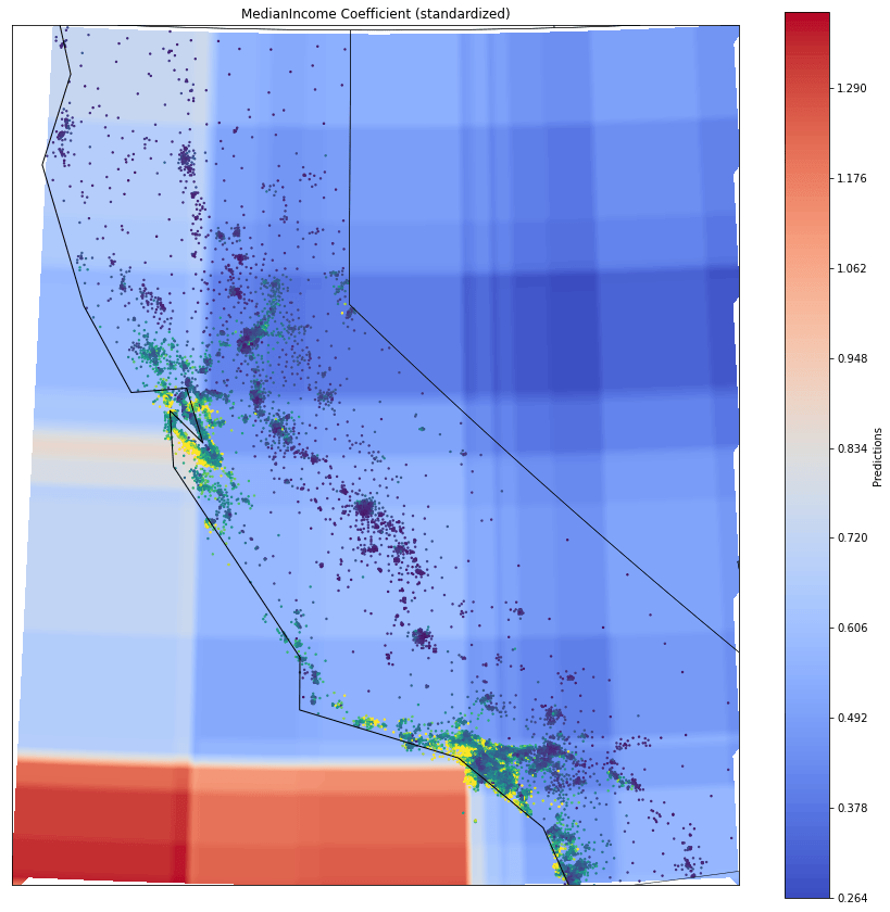
We see that the effect of MedInc is relatively stable throughout most of the area. In some coastal regions, particularly around Los Angeles and San Franscico, the effect of Median Income is slightly higher. Compare this to the estimated, coefficient according to the Varying Coefficient Neural Network:
# Predict using the model
predictions = model_net.predict_coefficients(torch.tensor(lat_lon_mesh).float())[:,1].detach().numpy()

# Create a basemap
m = Basemap(llcrnrlon=np.min(X_train_coeff[:, 1]), llcrnrlat=np.min(X_train_coeff[:, 0]),
            urcrnrlon=np.max(X_train_coeff[:, 1]), urcrnrlat=np.max(X_train_coeff[:, 0]),
            projection='lcc', lat_0=np.mean(X_train_coeff[:, 0]), lon_0=np.mean(X_train_coeff[:, 1]))

# Create a contour plot
plt.figure(figsize=(15, 15))
m.contourf(lon_mesh, lat_mesh, predictions.reshape(lat_mesh.shape), cmap='coolwarm',latlon=True, levels=200)
plt.colorbar(label='Predictions')
m.scatter(X[:, -1], X[:, -2], latlon=True, c=y, s=2)
m.drawcoastlines()
m.drawstates()
m.drawcountries()

plt.title('MedianIncome Coefficient (standardized; Neural Network estimate)')
plt.show()
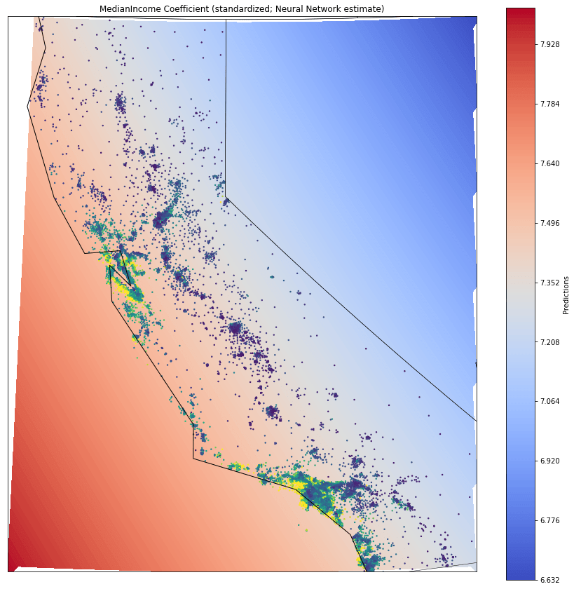
With the Varying Coefficient Neural Network, coefficient variation is much different from before. Instead of rectangular areas, the coefficients are now varying much more smoothly. This is obviously due to Neural Networks only being able to model smooth functions. Boosted Trees, on the other hand, can also account for non-smooth functions that change rapidly within a small area. With regard to geospatial data, this can obviously be limiting – here, for example, if neighborhood conditions change rather rapidly.
Nevertheless, the model also accounts for coastal homes’ prices being more influenced by Median Income.
Varying Coefficient Boosting for Bike Sharing Demand
Next up, we take a look at the Bike Sharing Demand dataset from Kaggle. The dataset contains hourly bike rental data from Washington D.C. Month, weekday, and hour are obviously key features here.
Thus, we take those as the inputs to our coefficient functions. To keep the feature count low, we apply cyclical encoding to hour, month and weekday:
bike_sharing = fetch_openml("Bike_Sharing_Demand", version=2, as_frame=True)
df = bike_sharing.frame

X = df.iloc[:,2:-1]
X["time"] = np.arange(len(X)) #add time axis for linear trend
y = df.iloc[:,-1]

X["month_sin"] = np.sin(2 * np.pi * X["month"] / 12)
X["month_cos"] = np.cos(2 * np.pi * X["month"] / 12)
X["hour_sin"] = np.sin(2 * np.pi * X["hour"] / 24)
X["hour_cos"] = np.cos(2 * np.pi * X["hour"] / 24)
X["weekday_sin"] = np.sin(2 * np.pi * X["weekday"] / 7)
X["weekday_cos"] = np.cos(2 * np.pi * X["weekday"] / 7)

X.drop(["month", "hour", "weekday"], axis=1, inplace=True)


# Create dummy variables for the specified columns
dummy_cols = ["holiday", "workingday", "weather"]
dummy_df = pd.get_dummies(X[dummy_cols], drop_first=True)

# Concatenate the dummy variables with the remaining columns
X = pd.concat([X.drop(dummy_cols, axis=1), dummy_df], axis=1)

X_train = X.iloc[:-1000]
X_test = X.iloc[-1000:]

y_train = np.log(y.iloc[:-1000]+1)
y_test = np.log(y.iloc[-1000:]+1)

data_features = ["weather_heavy_rain", "weather_misty", "weather_rain", "temp", "feel_temp", "humidity", "windspeed", "time", "holiday_False", "workingday_False"]

X_train_reg = np.float32(X_train[data_features])
X_train_coeff = np.float32(X_train.drop(data_features, axis=1))

X_test_reg = np.float32(X_test[data_features])
X_test_coeff = np.float32(X_test.drop(data_features, axis=1))

X_reg_mean = np.mean(X_train_reg, 0)
X_reg_std = np.std(X_train_reg, 0)

X_train_reg = (X_train_reg - X_reg_mean) / X_reg_std
X_test_reg = (X_test_reg - X_reg_mean) / X_reg_std

X_full_mean = np.mean(X_train, 0)
X_full_std = np.std(X_train, 0)

X_train_scaled = (X_train - X_full_mean) / X_full_std
X_test_scaled = (X_test - X_full_mean) / X_full_std

y_mean = np.mean(y_train)
y_std = np.std(y_train)

y_train = (y_train - y_mean) / y_std
y_test = (y_test - y_mean) / y_std
Let’s also repeat this with the Varying Coefficient Neural Network:
np.random.seed(123)
torch.manual_seed(123)

model_net = VaryingCoefficientNeuralNetwork(input_dim=X_train_reg.shape[1], varying_input_dim=X_train_coeff.shape[1], hidden_dim=10)
criterion = nn.MSELoss()
optimizer = optim.Adam(model_net.parameters(), lr=0.001)

model_net = VaryingCoefficientNeuralNetwork(input_dim=X_train_reg.shape[1]+1, varying_input_dim=X_train_coeff.shape[1], hidden_dim=10)
criterion = nn.MSELoss()
optimizer = optim.Adam(model_net.parameters(), lr=0.001)

X_train_reg_tensor = torch.tensor(X_train_reg).float()
X_train_reg_tensor = torch.cat([torch.ones(X_train_reg_tensor.shape[0], 1), X_train_reg_tensor], 1)

X_test_reg_tensor = torch.tensor(X_test_reg).float()
X_test_reg_tensor = torch.cat([torch.ones(X_test_reg_tensor.shape[0], 1), X_test_reg_tensor], 1)

X_train_coeff_tensor = torch.tensor(X_train_coeff).float()
X_test_coeff_tensor = torch.tensor(X_test_coeff).float()

y_train_tensor = torch.tensor(y_train).float()

num_epochs = 5000
for epoch in range(num_epochs):
    optimizer.zero_grad()
    outputs = model_net(X_train_reg_tensor, X_train_coeff_tensor)
    loss = criterion(outputs, y_train_tensor)
    loss.backward()
    optimizer.step()

predictions = model_net(X_test_reg_tensor, X_test_coeff_tensor)

rmse_var_coeff_net = np.sqrt(np.mean((predictions.detach().numpy() - y_test)**2))

print(f"RMSE for Varying Coefficient Boosting: {rmse_varcoeff}")
print(f"RMSE for Gradient Boosting: {rmse_gb}")
print(f"RMSE for varying coefficient Neural Network: {rmse_var_coeff_net}")
- RMSE for Varying Coefficient Boosting: 0.4491
- RMSE for Gradient Boosting: 0.4917
- RMSE for varying coefficient Neural Network: 0.4621
This time, the Varying Coefficient Boosting model even outperforms the standard Gradient Boosting model. Let us now compare how the Varying Coefficient Boosting model and the Varying Coefficient Neural Network model estimate the coefficient for the temp feature:
result_dict = {}

index = []
datalist = []

for hour in range(24):
    for month in range(12):
        for weekday in range(7):
            datalist.append([
                np.sin(2 * np.pi * hour / 24),
                np.cos(2 * np.pi * hour / 24),
                np.sin(2 * np.pi * month / 12),
                np.cos(2 * np.pi * month / 12),
                np.sin(2 * np.pi * weekday / 7),
                np.cos(2 * np.pi * weekday / 7),
            ])

            index.append(f"{hour+1},{month+1},{weekday+1}")


predictions_vcb = model._predict_coeffs(np.array(datalist))
predictions_vcnn = model_net.predict_coefficients(torch.tensor(np.array(datalist)).float()).detach().numpy()

for i in range(len(predictions)):
    result_dict[index[i]] = {"gb": f"{predictions[i,0]:.4f} + ... + {predictions[i,4]:.4f} * temp + ...",
                             "net": f"{predictions_vcnn[i,0]:.4f} + ... + {predictions_vcnn[i,4]:.4f} * temp + ..."}


result_dict_json = json.dumps(result_dict)

html_template = f"""
<!DOCTYPE html>
<html>
<head>
    <title>Model Selector</title>
</head>
<body>
    <label for="hour">Hour:</label>
    <input type="range" id="hour" name="hour" min="1" max="24" value="12" oninput="updateModel()">
    <span id="hourValue">12</span><br>

    <label for="month">Month:</label>
    <input type="range" id="month" name="month" min="1" max="12" value="8" oninput="updateModel()">
    <span id="monthValue">6</span><br>

    <label for="weekday">Weekday:</label>
    <input type="range" id="weekday" name="weekday" min="1" max="7" value="3" oninput="updateModel()">
    <span id="weekdayValue">3</span><br>

    <p>Varying Coefficient Boosting: <span id="vcbOutput"></span></p>
    <p>Varying Coefficient Neural Network: <span id="vcnnOutput"></span></p>

    <script>
        var modelData = {result_dict_json};

        function updateModel() {{
            var hour = document.getElementById('hour').value;
            var month = document.getElementById('month').value;
            var weekday = document.getElementById('weekday').value;

            document.getElementById('hourValue').textContent = hour;
            document.getElementById('monthValue').textContent = month;
            document.getElementById('weekdayValue').textContent = weekday;

            var vcbModelString = modelData[hour + ',' + month + ',' + weekday]['gb'];
            document.getElementById('vcbOutput').textContent = vcbModelString || 'No model available';
            var vcnnModelString = modelData[hour + ',' + month + ',' + weekday]['net'];
            document.getElementById('vcnnOutput').textContent = vcnnModelString || 'No model available';

        }}

        // Initial update
        updateModel();
    </script>
</body>
</html>
"""

with open('interactive_model_selector.html', 'w') as f:
    f.write(html_template)
6
3
Varying Coefficient Boosting:
Varying Coefficient Neural Network:
We find that the Varying Coefficient Network predict a negative temp coefficient at hour=12, month=8, weekday=3. On the contrary, the Varying Coefficient Boosting model appears to mostly predict a positive coefficient.
This might be a good occassion to ask a domain expert for their opinion. Then, we could fine-tune the varying coefficients by, for example, requiring the coefficient to be either all-negative or all-positive.
Taking Varying Coefficient Boosting further
Obviously, the models we were considering above were fairly generic. If we put in more effort to fully understand the data, we might come up with better suited models. In particular, we could do – for example – the following:
Constraining the coefficients’: As briefly mentioned, it might make sense to constrain the varying coefficients. If we knew, that certain coefficients have to be positive, we should definitely incorporate such prior knowledge. An  transformation could easily achieve this:
![\[\hat{y} = F^{(0)}(x) + \exp(F^{(1)}(x))\cdot x^{(1)} + \cdots F^{(M)}(x)\cdot x^{(M)},\]](https://sarem-seitz.com/wp-content/ql-cache/quicklatex.com-fd08bbf50adaf61a432462c757c9ff4b_l3.png "Rendered by QuickLaTeX.com")
presuming that  is the coefficient, we want to keep positive. Depending on your problem at hand, other constraints might be better suited.
Applying regularization: Just as in regression with fixed coefficients, we could add regularization terms to our loss function. This might be helpful if you are dealing with a high-dimensional dataset. As long as your regularization term is differentiable (as in, for example, Ridge Regression), PyTorch will give you the required gradients.
Keep in mind, though, that the standard theory for regularization considers fixed coefficients. Applying such methods to varying coefficients might yield unexpected results. Thus, you might want to do further research before using this idea in practice.
Keeping some coefficients constant: As our model is quite flexible, we might risk overfitting to some extent. The varying intercept term is particularly worrisome, as it is a standalone Gradient Boosting model already.
Therefore, you might want to keep some coefficients constant, rather than dynamic. To get an idea of how to do this, you might want to read this section of the previous article.
Using feature transformations in the regression formula: On the other hand, you might want to make your Varying Coefficient Boosting model even more flexible. If you were to consider feature transformations in a standard linear model, why not try them here as well.
Typical feature transformations are squares, logarithms or the harmonic transformation applied above.
Conclusion
By now, you have hopefully gotten an idea how useful varying coefficient models can be. Varying Coefficient Boosting is particularly interesting, as it allows for ‘rougher’ coefficient functions.
Even though the model is fairly transparent and interpretable, it does not cost too much performance. It is therefore a little unfortunate that there isn’t a respective mainstream Python package available yet.
Luckily, with the help of PyTorch, such approaches have become doable to build by yourself. If you need any help on that end, feel free to write a message or a comment below.
References
[1] Hastie, Trevor; Tishbirani, Robert. Varying-coefficient models. Journal of the Royal Statistical Society Series B: Statistical Methodology, 1993
[2] Yue, Mu; LI, Jialiang; Cheng, Ming-Yen. Two-step sparse boosting for high-dimensional longitudinal data with varying coefficients. Computational Statistics & Data Analysis, 2019
[3] Zhou, Yichen; Hooker, Giles. Decision tree boosted varying coefficient models. Data Mining and Knowledge Discovery, 2022
Leave a Reply